More details

read about the model different ways: High-Level, no math | More details, minimal math (this page) | All math

The first step is to estimate the distribution of participants in price space (more precisely, I’m estimating the distribution of guesses about future distribution of participants in log return space). Taking a window lagging the current time, I estimate this distribution using the price history.

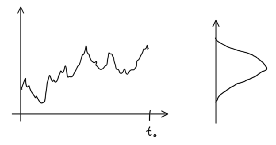
I’m making a number of assumptions here: there are participants where there are transactions; prices where there are many guesses show up more frequently in the price history; participants don’t consider volumes or use any weighting when making a guess about the distribution.

Next, I want to evolve that distribution forward in time so I can make a guess about the future. Think of this evolution like a function that takes the current distribution and produces a new one (the output will be roughly the same bell shape as the initial distribution, but with the width, peak(s), and tails slightly transformed; derivation here). There are unknown parameters in this function that determine e.g. how much the initial width matters, how sharp the peaks in the output are, etc. Based on many observations of initial and final distributions, I can find parameters that mazimize the likelihood of making those observations.

The really interesting part comes when I try to incorporate the influence of the market at large. I assume the same procedure, and estimate the distribution of participants in “expected return” space, i.e what participants want to get from any hypothetical investment. Then, adapting the evolution function so I can use this distribution as another input/output, I do the same parameter-fitting procedure. Rather than trying to use data across many markets for these observations, I do the following: I assume people are either 1) participating in the market of interest (the one where the underlying shares trade) or 2) not participating. By this definition, all people in my model universe are in one of the groups…at least in the short run. Then, I make a guess about how many have moved from 1) to 2) by comparing initial and final distributions for the market of interest (this is non-trivial. The information I want is actually related to the difference in the distribution of spatial frequencies…this leds to an interesting observation: I’m not modeling movement of some quantity of people, but an abstract quantity related to people’s guesses and the information available to them. For intuition about how spatial frequencies can be useful, imagine the surface of a lake on a calm day; compare that to the surface during a storm; the same amount of water may be there, but there is certainly another energy-like quantity that is absent on the calm day whose presence on the stormy day I can infer by looking at the size of the waves. This inference about the change in total “energy” is what I’m after). With guesses about the final distributions both in and out of the market of interest, I can proceed with the parameter-fitting procedure as usual.

The whole process looks something like this:

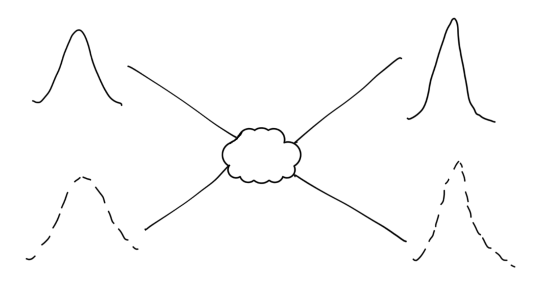
There is one distribution for everyone outside the market and one for everyone in it. The initial distributions “interact” and produce two final distributions.

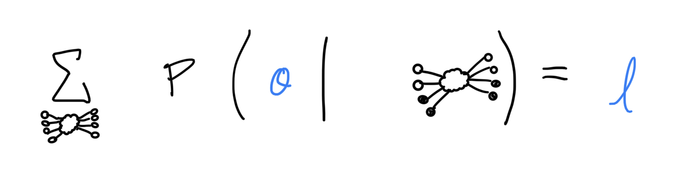
While the end goal is to estimate a distribution, the model estimates transition probabilities from an initial to a final price (log return). It is quite complicated to do this for an arbitrary number of participants. Instead, I can ask a simpler question about only one participant, drawn from the initial distribution, and use it to estimate the final distribution. That question is: “if I observe a participant transacting at price x now, how likely is it that I’ll see the same participant transacting at price y later?” In order to reconstruct a final distribution, I have to sample the initial distribution many times and sum up the transition probabilities for all possible y over all trials.

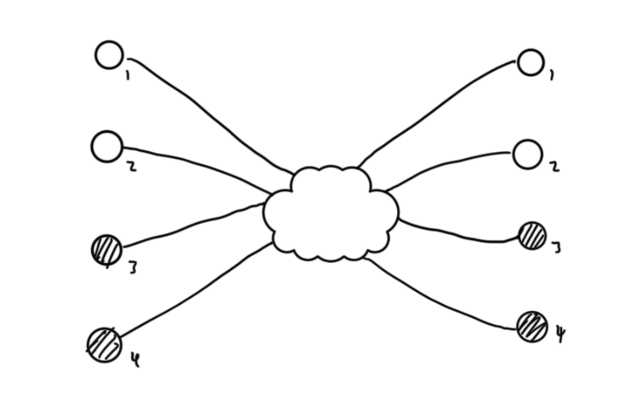
In fact, if I want to model the interaction of participants with other participants, I need to sample (at least) two participants at once and answer the joint question: “if I observe participants transacting at x₁ and x₂ now, how likely is it that I’ll see the same participants transacting at y₁ and y₂ later?” (Further, if I want to model interactions inside and outside the market, I need two participants from each for a total of four.)

Given an observation of initial distributions, I can choose any two points:

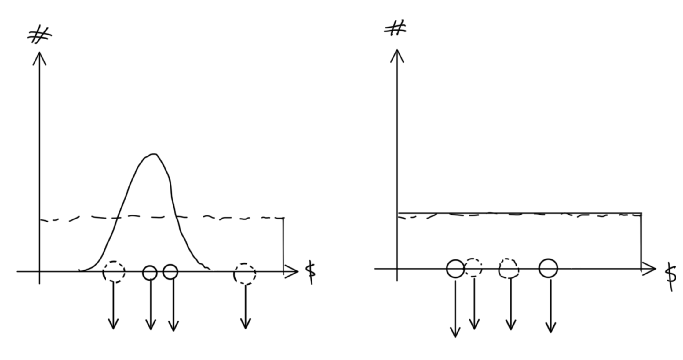
…let them “interact”:

…calculate the likelihood of the transition:

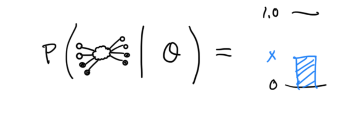
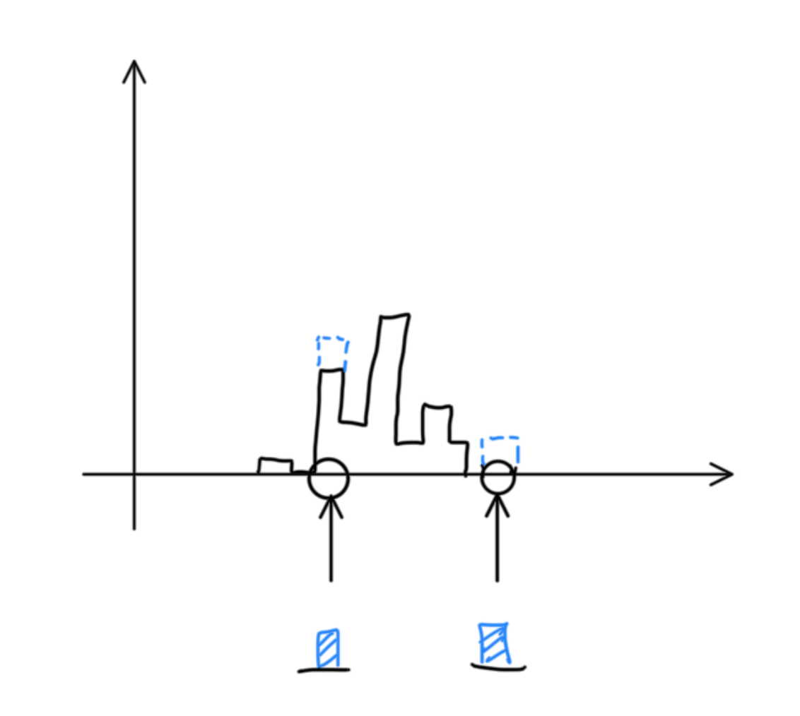
…then sum the likelihoods to get an estimate for the final distribution. (Note: I’m using “distribution” pretty loosely…but this model output is nonnegative and it can be normalized):

The training procedure, where I set the parameters of the model, is pretty similar. I perform the same sort of sampling and scoring for many possible pairs of initial/final samples across many different initial and final distributions (here, the final distributions are actually observed). The set of parameters used in the model is assigned a likelihood.

Then, the final task is to find set of parameters that maximizes the likelihood of observing the actual data. I used a MCMC procedure for this. Here’s how that goes: I start at some set of parameters, then take a random step in parameter space and accept the new values with a probability related to their likelihood. The steps will tend toward more likely values for the parameters. By assessing the size of the steps and the acceptance rate, I determine if the chain has “converged” on a region of high likelihood. The trace of the chain gives the joint likelihood distribution for the parameters. I pick the most likely set and fitting is complete!

Want even more math? Take me to Wonderland

Leave the rabbit hole? Get me out!